Introdutory workflow
This guide will walk you through a basic image stitching and analysis workflow in OpenHCS. By the end, you’ll understand how to set up a plate, create a stitching pipeline, and visualize results.
Step 1: Adding a Plate
What is a plate?
A plate (like a 96-well plate) contains multiple wells, each with multiple images (“fields”) at different positions. OpenHCS organizes images by this structure.
Supported formats: ImageXpress, Opera Phenix, OpenHCS ZARR (example dataset format)
Adding a plate:
For now, we will use a synthetic dataset included with OpenHCS. Under “View” in the main menu, click “Generate Synthetic plate”, or click Ctrl+Shift+G. Click confirm in the dialog that appears.
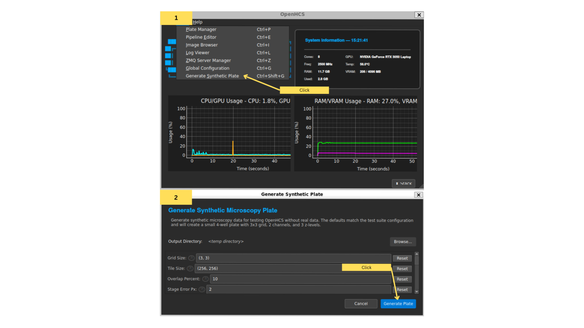
This creates a synthetic plate with random data, and creates a sample stitching + analysis pipeline. Hit “Init” in the plate manager to initialize the plate.
Uploading your own data
For reference, if you’d rather upload your own dataset, follow these steps:
Open Plate Manager
Click “Add” → navigate to your dataset folder → “Choose”
OpenHCS will auto-detect the format and load it
Click “Init” to initialize
Open the pipeline editor
Step 2: Exploring the Image Browser & Metadata Viewer
Image Browser
The Image Browser lets you view and explore images in your plate. Click on “Meta” in the plate manager to open it. (Note: This wont work unless you’ve initialized a plate first. Hit the “Init” button if the Meta button is greyed out).
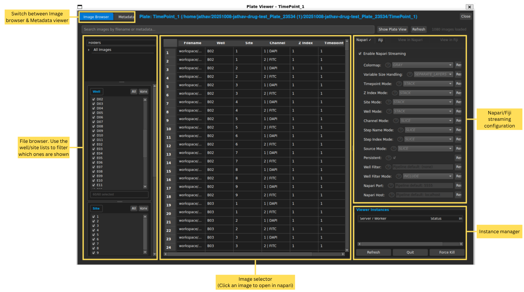
In the Image Browser, you can navigate through the different wells and fields of your plate, and view the images associated with each one.
This table in the middle shows all images in the plate. You can filter images by well, field, channel, timepoint, etc. using the filters on the left. On the right, the configuration for either the Napari or Fiji streaming viewer can be adjusted. For details on each configuration option, refer to Configuration Reference, or hover over the (?) button next to each option for a tooltip.
Metadata Viewer
If you switch to the “Metadata” tab at the top, you can view metadata associated with your images, such as acquisition settings, experimental conditions, and annotations, as well as edit it.
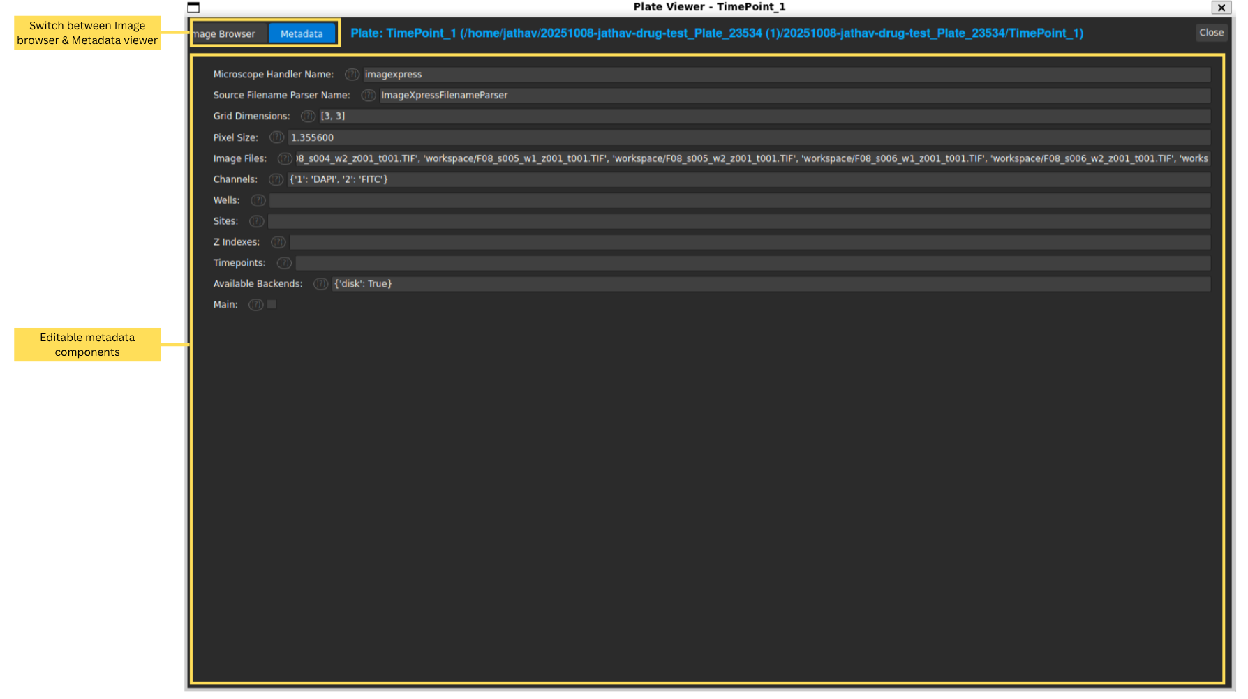
In the Metadata tab, you can view and edit metadata associated with your images, such as grid dimensions, channels, and other experimental details.
Now, let’s look at how to do things with these images. Open the Pipeline editor by clicking view on the main menu and clicking “Pipeline Editor”.
Step 3: Setting up a Stitching Pipeline
Understanding Pipelines
A pipeline is a sequence of steps that process your images in a specific order. Think of it like a laboratory protocol.
Each pipeline is made of multiple steps. A step in OpenHCS is a single operation. This doesn’t mean they only do one thing, however. Many steps perform multiple operations.
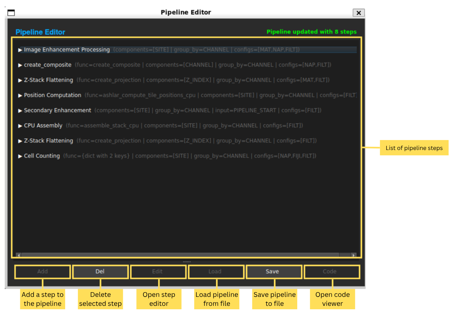
The Pipeline Editor shows the sequence of steps that make up your image processing workflow.
Tip: Sharing/Importing Pipelines
The best way to share pipelines is by clicking the “Code” button and copying the generated code. Anyone else can paste it into their own code viewer and load your pipeline, and vice versa.
Steps and the Step Editor
Lets take a look at a individual step by opening the Step Editor. Double-click on the first step in the pipeline (named “Image Enhancement Processing”) to open it.
There are 2 tabs in the Step Editor: “Step Settings” and “Function Pattern”. Lets look at step settings for now.
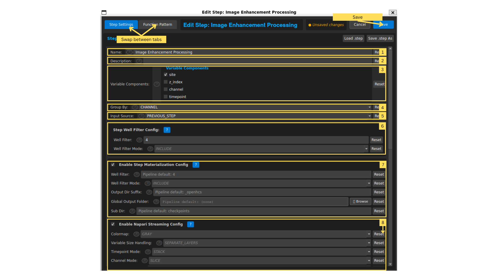
Step Name: This is the name of the step. You can change it to something more descriptive if you want.
Step Description: A brief description of what this step does.
Variable Components:
These tell OpenHCS how to split up images before processing.
Typical image microscopy plates have many “dimensions”, such like which well they came from, which site in the well, which wavelength channel (DAPI, FITC, TL-20), which timepoint (for live imaging), or which z-dimension it was on (for 3D image, commonly reffered to as a “z-stack”).
OpenHCS groups images into “piles” based on the variable components you select. Each pile is processed separately.
The variable component you choose determines which variable changes within a pile. All other dimensions (not selected as variable components) remain the same within that pile.
OpenHCS will create a separate pile for every unique combination of the non-variable dimensions.
In this example, the variable component is the site. The other dimensions are well and channel. This means that for each well and channel combination, there will be a seperate pile, and within each pile, the only difference between images is the site. So, for well A1 and channel ‘Wavelength 1’, there will be a pile with an image for each site. There will be another pile for well A1 and channel ‘Wavelength 2’, again with images for each site, and so on.
Extra help
If that doesn’t make sense, think about it this way: Imagine you’re a teacher with exam papers from multiple classes (Class A, B, C), multiple sections (Math, Science, English), multiple time periods (Morning, Evening), and multiple seat numbers (1-30) in each class.
If you select “Time period” as your Variable Component:
You’d create separate piles for each class, section and seat number combination
Within each pile, all papers will have the same class, subject, and seat number — only the time period will differ.
For example: One pile might have all papers from Class A, Seat #1, across all sessions
Another pile would have Science papers from Class B, seat #15, and so on.
In our microscopy example where “site” is the Variable Component:
We create separate processing groups where only the site varies
Each group contains images from all sites of a specific channel of a specific well
This is done because sometimes the processing we want to do (like stitching) needs to consider all sites together for each well and channel. Or, we might want to have our variable component be channel so that we can compare how different fluorescence markers look in the same well and site.
Group By
This tells OpenHCS how to treat variations inside each group.
In other words, after the images have been split into groups (using Variable Components), Group By decides what differences still matter inside those groups.
For example, in this example we want to process each channel differently: our Wavelength 1 channel need different filtering than our Wavelength 2 channel. So we “Group By” channel.
Extra help
If that doesn’t make sense, think about it this way:
Imagine you’re a teacher with exam papers from multiple classes (Class A, B, C), multiple sections (Math, Science, English), multiple time periods (Morning, Evening) , and multiple seat numbers (1-30) in each class.
You want to process each subject individually because the grading rules differ. So, you “Group By” subject within each class pile, and use a different answer key to mark each test.
Similarly, in OpenHCS, you might want to vary your analysis based on which fluorescence markers you stained with.
Input Source: Which images are being used (previous step output or original plate images);
Step Well Filter: Process only specific wells (e.g., A1 and B1). Leave blank to process all wells.
Materialization Config: Save intermediate results to disk (inherits from global config unless changed).
Napari/Fiji Streaming Config: Visualize step results in Napari or Fiji (inherits from global config as well).
For more details on each configuration option, refer to Configuration Reference, or hover over the (?) button next to each option for a tooltip.
Function Pattern Tab
Hit save to close this step’s editor. Open the step named “Cell Counting”, and then click “Function Pattern” at top. A step’s function pattern is its series of operations.
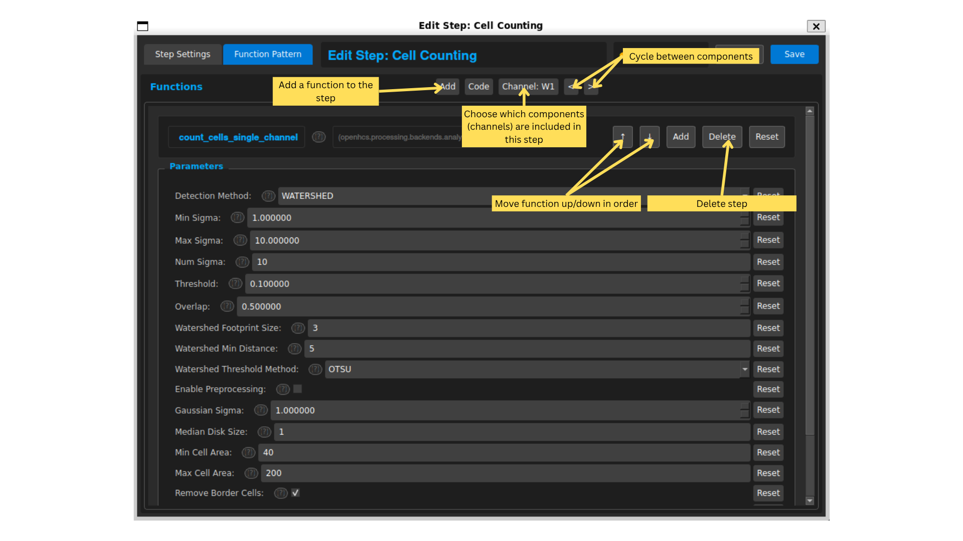
This step runs a cell counting analysis on images. The function pattern shows the sequence of functions applied to the images in this step. Steps can include multiple functions, but typically you should just have one main function per step for clarity.
Note: The component you can cycle through/select is the component selected to “Group By” in the step settings. You can change what functions are applied to each component by cycling through them using the arrows at top-right.
Pipeline Overview
Now that we’ve explored one step, let’s look at the overall pipeline. This pipeline is designed for stitching and analyzing images. It processes images, stitches them together, and then analyzes the stitched images to extract useful information (in this case, it runs a simple cell-counting analysis on the stitched images).
The pipeline consists of the following steps:
Image Enhancement Processing: Prepares images for stitching by applying filters.
Create Composite With the variable component as channel, this step creates a composite image using both channels for each site of each well of each z-stack, so that there is only 1 image for each position. This is needed because stitching requires just one image per position, but with multi-channel images, there are multiple images per position (one for each channel).
Z-Stack Flattening This does the same as Create Composite, but for z-stacks (3d heights). It flattens multiple z-slices into a single 2D image per position.
Position Computation: Computes the positions of each image for stitching.
Secondary Enhancement: Further enhances images post-stitching. We do a second processing step because the stitching process prefers different image characteristics than analysis steps do. Note that this step takes the original images as input, not the stitched images.
CPU assembly: Stitches images together based on computed positions from step 4, using images from step 5.
Z-Stack Flattening: Flattens z-stacks of stitched images into single 2D images. We do this to make the final analysis better.
Simple Cell Counting Analysis: Analyzes the stitched images to count cells and extract statistics.
Conclusion
You can try running the pipeline now to see how it performs. To run a pipeline, hit “Compile”, and then “Run”. You can modify where the output goes to in the plate configuration, by hitting edit on the plate manager. See Configuration Reference for details on changing output directories and other configurations.
The steps described above cover the simplest stitch and analyze workflow and will be suitable for most projects — just add any extra analysis steps you need for your experiment, and tweak image processing filters in Steps 1 and 5 as needed. You also might need to add/remove compositing or z-flattening steps depending on what variable components your data has available.
If you encounter major issues, regressions, or missing features, please open an issue on the project’s GitHub with a short description, reproduction steps, and any relevant logs or sample data. (Link: https://github.com/trissim/openhcs/issues)